Introduction to Stochastics – A Look at Monte Carlo Method and Hidden Markov Model

Note: This is a paper I wrote for my AH Computer Science course, hence the formality.

Preface

A stochastic process is a process that involves aggregating results to find patterns in an otherwise random-seeming phenomena. Sometimes we can’t determine exact functions for representing complicated events or processes and rather than assuming everything is arbitrary and random, mathematicians and computer scientists have developed algorithms for modeling these processes and determining trends. While the models tend not to be consistent exactly with reality, as they are simplifying assumptions, they do help us determine trends in things that we would otherwise think are random processes.

The Hidden Markov Model and Monte Carlo Method are two different ideas in computer science with a connected goal of determining algorithms although they solve different problems. The Hidden Markov Model is a model developed to understand processes where the effects can be observed but the algorithm is unknown. The hidden process is referred to as the “Markov Process,” and the model is the graphical interpretation of the possible algorithms. The Monte Carlo Method is a class of algorithms rather than a model for visualizing possible processes. The algorithms are designed to compute values that are generally not easy to find via a function through probabilistic sampling. These algorithms, while part of a broad category, follow a general structure of taking a domain of possible input values with probabilities of these values occurring and then using a “deterministic algorithm” (an algorithm that takes gives a unique output for each unique input) to find individual results. The idea is that aggregating all of the algorithm results will maintain some sort of consistent behavior with which we can use to determine the behavior of the object for which the Monte Carlo algorithm was designed.

Hidden Markov Process

There are a few definitions surrounding what a Markov Process is. A Markov Process is not solely a hidden algorithm. It’s an algorithm that, at each state of the algorithm, we are able to determine the entire history of the algorithm (Ghahramani). For example, consider speech. A person talks with a non-random string of words (because humans cannot be random). We don’t know for certain what word will come next but we can use the previous words to make a guess as to what will come next. This is a Markov Process.

Hidden Markov Model

The HMM is a model for visualizing a Markov Process. Instead of delving into the mathematics, I will first illustrate how this model works by showing a few examples.

Observe this schematic

Here is an example of the Hidden Markov Model that I came up with. Let’s say Spencer is in a room with n different dictionaries, each of the same language. The problem is that each definition within each dictionary is unique. We don’t know how they are unique but we know that each dictionary has a random assortment of definitions although they all contain the same words. Alex is on the outside of the room. Spencer, with an unknown algorithm, chooses a definition from any of the dictionaries and sends out to Alex to determine which dictionary it came from so he can find what word it is. Alex has no way of figuring out how Spencer is choosing definitions but can say with a certain probability, specifically 1/n, which dictionary it is coming from. Spencer continues with this process and over a finite period of time, Alex will be able to determine the algorithm through probabilistic interpolation.

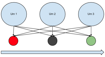
An example given on Wikipedia is that there is a room with a conveyor belt leading out. A genie is within the room with n urns containing some assortment of colored balls and has a hidden Markov Process or unknown algorithm for sending the balls out of the room. An observer, we’ll say Peter, is outside observing the stream of colored balls exiting the room. He can’t determine what algorithm the genie is using because he doesn’t know from which urns the colored balls are coming from (because the colored balls exist in all possible urns). But he can make probability guesses as to figure out what the algorithm is. Consider the following schematic on the left. The long arrow indicates direction while the arrows from urns to the colored circles indicate possible ball orderings. One aspect about the Markov Process is that the genie’s choice of next urn is dependent on the present urn.

Monte Carlo Method**

**

The Monte Carlo Method is a class of algorithms based on random sampling. Based on the statistical idea that a near-infinite quantity (yet finite) of tests will reveal a pattern and if a near-infinite quantity of tests doesn’t reveal a pattern, we can conclude that it is a random procedure.

Let’s say you want to find the value of pi. The ratio of the area of a circle to the area of a square with a side length congruent to the radius of the circle is equal to pi. So we place the square within the circle and proceed to throw grains of rice, each of unit area 1, onto the circle-square body. We continue with this random sampling of points, all the while taking the ratio of number of rice grains outside of the square and within the square to the number of rice grains found within the square. This ratio will be very close to pi once both the square and circle are covered in rice grains.

An important aspect of the Monte Carlo Method is that these algorithms tend to follow a general procedure:

1. Given a domain of possible inputs, determine each input’s probability of being chosen
2. Use a deterministic algorithm to sample each input and record the output
3. Aggregate the outputs

The Monte Carlo Method allows computers to quickly calculate all possible outcomes within a reasonable time period. This is a useful procedure especially in situations where there exists uncertainty to human perspective but a computer can visualize with probabilities all risky outcomes.

The Monte Carlo Method is one of the defining algorithms of stochastics as it depends on aggregating results from a model.

Monte Carlo Algorithm Examples

Here is an example I thought of while driving. Let’s say you throw a handful of sand onto a sidewalk and you want to determine each grain’s location. You could start with looking at each sand grain’s trajectory, factoring in its mass and its direction by projecting the grains into three-dimensional space. You could then account for the various directions of forces acting on the flying sand grains. This is wildly unrealistic given all of the anomalous forces that could affect a tiny sand grain, including the gravitational force of every sand grain on each other. We have to simplify the forces acting on the grains of sand but let’s say we reduce it to several thousand varying forces. So, with a rather long calculation (somewhat long for a computer to calculate trajectories for a thousand sand grains in three-dimensional space) we can estimate the locations of grains of sand.

An alternate way, by using the Monte Carlo Method, ignores all varying forces that could be acting on the grains of sand. Here is the algorithm I propose:

1. Assume that all of the anomalous forces are not anomalous but consistent with every trial. Similarly, assume that all external factors are held constant, each handful of sand is equal in mass and volume to the next, and each throw is consistent. These are reasonable assumptions given that external factors don’t vary much, grains of sand are close to being the same, and each throw can be made consistent. Similarly, we are only searching for an estimate, not an exact calculation. Finally, we assume that each grain of sand corresponds to another grain in a consecutive trial. These grains have the same initial trajectory.
2. Take a handful of sand and throw it. Record the locations in 2-d space of all grains of sand.
3. Clear sidewalk and repeat step 1 until you’ve collected enough results, whatever “enough” is in your definition. I would say several hundred thousand.
4. Aggregate the results by averaging the positions of each grain of sand based on their initial trajectory.

We should be able to estimate where grains of sand will land given certain conditions because of repeated analysis.

In general though, Monte Carlo Methods aren’t straight-up repeated aggregations of experiments. Sometimes there exist models which are repeatedly tested until a general pattern emerges.

Applications of the Hidden Markov Model & Monte Carlo Method

A Hidden Markov Model is a way of modeling a Hidden Markov Process or an algorithm that cannot be viewed except for its output states. Examples of Hidden Markov Processes include speaking, weather, and financial forecasting. We can use models that view the previous outputs and then extrapolate or predict the next output based off of certain probabilities. The Hidden Markov Model can be used in many different contexts, ranging from AI video game design to stock market predictions. Yet, while the HMM is a surprisingly simple concept, applying it can range in complexity. Generally, applications of the Hidden Markov Model require a physical knowledge of the phenomena that the system describes. For example, if I wanted to design an algorithm to predict stock market movement, I would have to physically determine a relationship between market behavior and its past few states.

A connection between the Hidden Markov Model and the Monte Carlo Method is that the HMM relies on a physical correlation to be clear while the Monte Carlo Method can determine a physical correlation via random sampling tests. Let’s say we have a model for a Hidden Markov process but we don’t have a physical relationship (like numbers corresponding to probabilities, etc…), we can use the Monte Carlo Method based on the model to derive probabilities via random sampling. If we have a process that we think we have modeled, and would like to determine the physical correlation, we could run the model many, many times and aggregate the results. The results would then show a probability trend distributed over the tests which we could then use in conjunction with the Hidden Markov Model to definitively determine and implement an algorithm or computer software that predicts process outputs.

The Monte Carlo Method isn’t solely for procedures with hidden algorithms or processes. But, it is used when computing a trend or exact value is not evident, timely, or possible within a reasonable time period. It’s easy to run repeated tests and aggregate results, but it is not easy to determine theoretical answers to problems via logical reasoning. Its myriad applications include everything from investment analysis to operations research.

Introduction to Stochastics

The Hidden Markov Model and the Monte Carlo Method are both part of a discipline known as stochastics. Stochastics is the science of determining or predicting future states with a given probability. While we cannot be one hundred percent certain about future events, we can try to determine the probability (and to a greater extent, the certainty) behind a given phenomena. The Hidden Markov Model is a way of correlating outputs with a hidden process and the Monte Carlo Method is a way of determining patterns in processes that are seemingly impossible to compute or determine. The Monte Carlo Method requires a model to run tests on (which could be the Hidden Markov Model) while the Hidden Markov Model is a way of representing the connection between hidden algorithms and their outputs. These two ideas are fundamental to the discipline of stochastics and have wide applications ranging from bioinformatics, finance, linguistics, and meteorology.

Stochastics is a wide field extending into a variety of human and scientific disciplines. Essentially, it is the science of uncertainty, randomness, and probability. The Monte Carlo Method and the Hidden Markov Model are two fundamental ideas in stochastics. Yet, these two ideas are very wide-reaching and contain many different sub-categories for research and software development. When designing software that deals with physically random phenomena, the Monte Carlo Method and Hidden Markov Model are two approaches to use when modeling and designing algorithms to achieve physical results.

Works Cited

http://mlg.eng.cam.ac.uk/zoubin/papers/ijprai.pdf

http://www.cs.umd.edu/~djacobs/CMSC828/ApplicationsHMMs.pdf

http://statweb.stanford.edu/~owen/mc/Ch-intro.pdf

http://en.wikipedia.org/wiki/Hidden_Markov_model

https://www.ma.utexas.edu/users/gordanz/notes/introduction_to_stochastic_processes.pdf